Daily statistics from hourly ERA5 data
[1]:
from earthkit import data as ekd
from earthkit import plots as ekp
from earthkit import transforms as ekt
from earthkit.transforms._tools import earthkit_remote_test_data_file
Load some test data
All earthkit-transforms methods can be called with earthkit-data objects (Readers and Wrappers) or with the pre-loaded xarray.
In this example we will use hourly ERA5 2m temperature data on a 0.5x0.5 spatial grid for the year 2015 as our physical data.
First we download (if not already cached) lazily load the ERA5 data (please see tutorials in earthkit-data for more details in cache management).
We convert the data to an xarray.Dataset with some additional options which are better suited for the data we are working with.
[2]:
# Get some demonstration ERA5 data, this could be any url or path to an ERA5 grib or netCDF file.
remote_era5_file = earthkit_remote_test_data_file("era5_temperature_europe_2015.grib")
era5_xr = ekd.from_source("url", remote_era5_file)
era5_xr = era5_xr.to_xarray(time_dims=["valid_time"]).rename({"2t": "t2m"})
era5_xr
[2]:
<xarray.Dataset> Size: 660MB
Dimensions:     (valid_time: 1460, latitude: 201, longitude: 281)
Coordinates:
  * valid_time  (valid_time) datetime64[us] 12kB 2015-01-01 ... 2015-12-31T18...
  * latitude    (latitude) float64 2kB 80.0 79.75 79.5 79.25 ... 30.5 30.25 30.0
  * longitude   (longitude) float64 2kB -10.0 -9.75 -9.5 ... 59.5 59.75 60.0
Data variables:
    t2m         (valid_time, latitude, longitude) float64 660MB ...
Attributes:
    Conventions:  CF-1.8
institution: ECMWFCalculate the daily mean and standard deviation of the ERA5 data
We can calculate the daily mean using daily_mean method in the temporal module. There are similar daily aggregation methods for the daily_median, daily_min, daily_max, daily_std, daily_sum, and all these again for monthly aggregations in the form monthly_XXX.
earthkit-aggregate is able to understand any data object understood by earthkit-data as input. The earthkit-aggregate computation is based on xarray datacubes, therefore the returned object is an xarray.Dataset. To convert this to an EarthKit object you could use the earthkit-data method, from_object.
If the input data is provided an xarray.Dataset then the return object is xarray.Dataset and if the input is an xarray.DataArray then the return object is an xarray.DataArray.
[3]:
era5_daily_mean = ekt.temporal.daily_mean(era5_xr)
era5_daily_std = ekt.temporal.daily_std(era5_xr)
era5_daily_mean
[3]:
<xarray.Dataset> Size: 165MB
Dimensions:     (valid_time: 365, latitude: 201, longitude: 281)
Coordinates:
  * valid_time  (valid_time) datetime64[us] 3kB 2015-01-01 ... 2015-12-31
  * latitude    (latitude) float64 2kB 80.0 79.75 79.5 79.25 ... 30.5 30.25 30.0
  * longitude   (longitude) float64 2kB -10.0 -9.75 -9.5 ... 59.5 59.75 60.0
Data variables:
    t2m         (valid_time, latitude, longitude) float64 165MB 254.4 ... 285.8
Attributes:
    Conventions:  CF-1.8
institution: ECMWFCalculate the monthly mean and standard deviation
[4]:
era5_monthly_mean = ekt.temporal.monthly_mean(era5_xr)
era5_monthly_std = ekt.temporal.monthly_std(era5_xr)
era5_monthly_std
[4]:
<xarray.Dataset> Size: 5MB
Dimensions:     (valid_time: 12, latitude: 201, longitude: 281)
Coordinates:
  * valid_time  (valid_time) datetime64[us] 96B 2015-01-01 ... 2015-12-01
  * latitude    (latitude) float64 2kB 80.0 79.75 79.5 79.25 ... 30.5 30.25 30.0
  * longitude   (longitude) float64 2kB -10.0 -9.75 -9.5 ... 59.5 59.75 60.0
Data variables:
    t2m         (valid_time, latitude, longitude) float64 5MB 6.104 ... 6.375
Attributes:
    Conventions:  CF-1.8
institution: ECMWFCalculate a rolling mean with a 50 timestep window
To calculate a rolling mean along the time dimension you can use the rolling_reduce function.
NOTE: An improved API to the rolling_reduce method is an ongoing task
[5]:
era5_rolling = ekt.temporal.rolling_reduce(
    era5_xr,
    50,
    how_reduce="mean",
    center=True,
)
era5_rolling
[5]:
<xarray.Dataset> Size: 660MB
Dimensions:     (valid_time: 1460, latitude: 201, longitude: 281)
Coordinates:
  * valid_time  (valid_time) datetime64[us] 12kB 2015-01-01 ... 2015-12-31T18...
  * latitude    (latitude) float64 2kB 80.0 79.75 79.5 79.25 ... 30.5 30.25 30.0
  * longitude   (longitude) float64 2kB -10.0 -9.75 -9.5 ... 59.5 59.75 60.0
Data variables:
    t2m         (valid_time, latitude, longitude) float64 660MB dask.array<chunksize=(1459, 26, 36), meta=np.ndarray>
Attributes:
    Conventions:  CF-1.8
institution: ECMWFAccount for non-UTC timezones
There is a time_shift argument which can be used to account for non-UTC time zones:
[6]:
era5_daily_mean_p12 = ekt.temporal.daily_mean(era5_xr, time_shift={"hours": 12})
era5_daily_mean_p12
[6]:
<xarray.Dataset> Size: 165MB
Dimensions:     (valid_time: 366, latitude: 201, longitude: 281)
Coordinates:
  * valid_time  (valid_time) datetime64[us] 3kB 2015-01-01 ... 2016-01-01
  * latitude    (latitude) float64 2kB 80.0 79.75 79.5 79.25 ... 30.5 30.25 30.0
  * longitude   (longitude) float64 2kB -10.0 -9.75 -9.5 ... 59.5 59.75 60.0
Data variables:
    t2m         (valid_time, latitude, longitude) float64 165MB 253.5 ... 285.6
Attributes:
    Conventions:  CF-1.8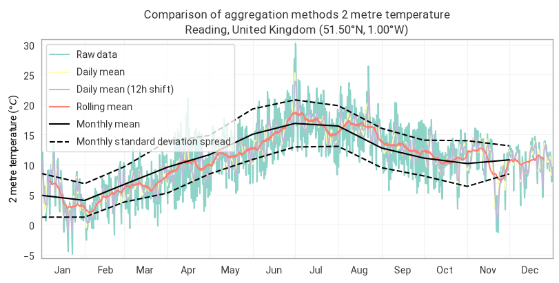
institution: ECMWFPlot a random point location to see the different aggregation methods
[7]:
latitude = 51.5
longitude = -1.0
sel_kwargs = {"latitude": latitude, "longitude": longitude}

chart = ekp.TimeSeries()

# Plot the raw data and various aggregations on the same chart for comparison:
# Raw data:
chart.line(era5_xr.sel(**sel_kwargs), units="celsius", label="Raw data")
# Daily mean:
chart.line(era5_daily_mean.sel(**sel_kwargs), units="celsius", label="Daily mean")
# Daily mean with 12h shift:
chart.line(era5_daily_mean_p12.sel(**sel_kwargs), units="celsius", label="Daily mean (12h shift)")
# Rolling mean:
chart.line(era5_rolling.sel(**sel_kwargs), units="celsius", label="Rolling mean")

# Add the monthly mean as a black solid line and spread as black dotted lines:
chart.line(era5_monthly_mean.sel(**sel_kwargs), units="celsius", label="Monthly mean", color="black")
upper_m = era5_monthly_mean + era5_monthly_std
lower_m = era5_monthly_mean - era5_monthly_std
chart.line(
    upper_m.sel(**sel_kwargs),
    units="celsius",
    label="Monthly standard deviation spread",
    linestyle="--",
    color="black",
)
chart.line(lower_m.sel(**sel_kwargs), units="celsius", linestyle="--", color="black")

chart.title(
    "Comparison of aggregation methods {variable_name}\n{location:%c}, {location:%C} ({latitude:%Lt}, {longitude:%Ln})"
)

chart.ylabel()

chart.xticks(frequency="M", format="%b", period=True)

chart.legend()

chart.show()
[ ]: