Masking data-cubes using geometry objects
[1]:
from earthkit import data as ekd
from earthkit import plots as ekp
from earthkit import transforms as ekt
from earthkit.transforms._tools import earthkit_remote_test_data_file
Load some test data
All earthkit-transforms methods can be called with earthkit-data objects or with pre-loaded xarray or geopandas objects.
In this example we will use hourly ERA5 2m temperature data on a 0.5x0.5 spatial grid for the year 2015 as our physical data; and we will use the NUTS geometries which are stored in a geojson file. As we are going to repeat calls to the aggregation methods, we will convert the data to xarray.Dataset and geopandas to avoid repeated conversion.
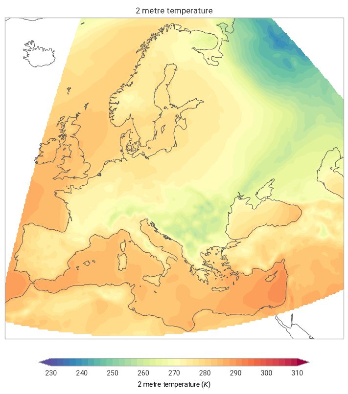
The cells below downloads some sample ERA5 data and opens as an xarray object (first cell), then plots the data using earthkit.plots.
[2]:
# Get some demonstration ERA5 data, this could be any url or path to an ERA5 grib or netCDF file.
# remote_era5_file = earthkit_remote_test_data_file("era5_temperature_europe_2015.grib") # Large file
remote_era5_file = earthkit_remote_test_data_file("era5_temperature_europe_20150101.grib")
era5_data = ekd.from_source("url", remote_era5_file)

# Open as an xarray dataset, renaming the 2m temperature variable to something more manageable
era5_xr = era5_data.to_xarray(time_dims=["valid_time"]).rename({"2t": "t2m"})
era5_xr
[2]:
<xarray.Dataset> Size: 11MB
Dimensions:     (valid_time: 24, latitude: 201, longitude: 281)
Coordinates:
  * valid_time  (valid_time) datetime64[us] 192B 2015-01-01 ... 2015-01-01T23...
  * latitude    (latitude) float64 2kB 80.0 79.75 79.5 79.25 ... 30.5 30.25 30.0
  * longitude   (longitude) float64 2kB -10.0 -9.75 -9.5 ... 59.5 59.75 60.0
Data variables:
    t2m         (valid_time, latitude, longitude) float64 11MB ...
Attributes:
    Conventions:  CF-1.8
institution: ECMWF[3]:
ekp.geo.plot(era5_xr.mean(dim="valid_time"), domain="Europe")
/home/docs/checkouts/readthedocs.org/user_builds/earthkit-transforms/envs/1.0.0/lib/python3.11/site-packages/cartopy/io/__init__.py:242: DownloadWarning: Downloading: https://naturalearth.s3.amazonaws.com/50m_physical/ne_50m_coastline.zip
  warnings.warn(f'Downloading: {url}', DownloadWarning)
[3]:
<earthkit.plots.components.maps.Map at 0x76da8f3d9f90>
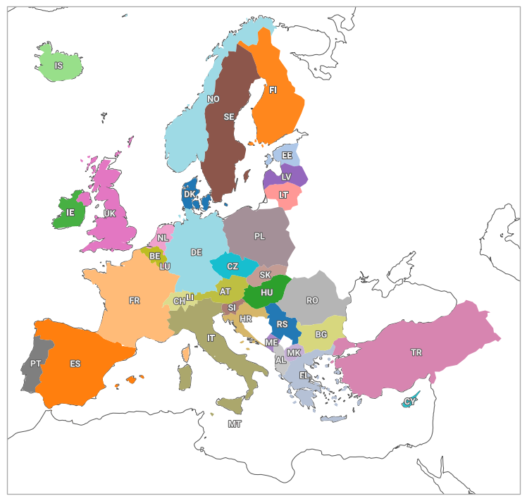
We do the same for our geojson data, except this time we open as a geopandas objects and plot using the built in geopandas methods.
[4]:
# Use some demonstration polygons stored, this could be any url or path to geojson file
remote_nuts_url = earthkit_remote_test_data_file("NUTS_RG_60M_2021_4326_LEVL_0.geojson")
nuts_data = ekd.from_source("url", remote_nuts_url).to_geopandas()

nuts_data[:5]
[4]:
| id | NUTS_ID | LEVL_CODE | CNTR_CODE | NAME_LATN | NUTS_NAME | MOUNT_TYPE | URBN_TYPE | COAST_TYPE | FID | geometry | |
|---|---|---|---|---|---|---|---|---|---|---|---|
| 0 | DK | DK | 0 | DK | Danmark | Danmark | 0 | 0 | 0 | DK | MULTIPOLYGON (((15.1629 55.0937, 15.094 54.996... |
| 1 | RS | RS | 0 | RS | Serbia | Srbija/Сpбија | 0 | 0 | 0 | RS | POLYGON ((21.4792 45.193, 21.3585 44.8216, 22.... |
| 2 | EE | EE | 0 | EE | Eesti | Eesti | 0 | 0 | 0 | EE | MULTIPOLYGON (((27.357 58.7871, 27.6449 57.981... |
| 3 | EL | EL | 0 | EL | Elláda | Ελλάδα | 0 | 0 | 0 | EL | MULTIPOLYGON (((28.0777 36.1182, 27.8606 35.92... |
| 4 | ES | ES | 0 | ES | España | España | 0 | 0 | 0 | ES | MULTIPOLYGON (((4.391 39.8617, 4.1907 39.7981,... |
[5]:
ekp.geo.choropleth(nuts_data, z=None, labels="FID", domain="Europe").show()
[5]:
<earthkit.plots.components.figures.Figure at 0x76da8f3b18d0>
Mask data with the geometries
shapes.mask applies the features in the geometry object (nuts_data) to the data object (era5_data). It returns an xarray object with an additional dimension, and coordinate variable, corresponding to the features in the geometry object. By default this is the index of the input geodataframe, in this example the index is just an integer count so it takes the default name index.
[6]:
masked_data = ekt.spatial.mask(era5_xr, nuts_data)
masked_data
[6]:
<xarray.Dataset> Size: 401MB
Dimensions:     (index: 37, valid_time: 24, latitude: 201, longitude: 281)
Coordinates:
  * index       (index) int64 296B 0 1 2 3 4 5 6 7 8 ... 29 30 31 32 33 34 35 36
  * valid_time  (valid_time) datetime64[us] 192B 2015-01-01 ... 2015-01-01T23...
  * latitude    (latitude) float64 2kB 80.0 79.75 79.5 79.25 ... 30.5 30.25 30.0
  * longitude   (longitude) float64 2kB -10.0 -9.75 -9.5 ... 59.5 59.75 60.0
Data variables:
    t2m         (index, valid_time, latitude, longitude) float64 401MB dask.array<chunksize=(1, 24, 201, 281), meta=np.ndarray>
Attributes:
    Conventions:  CF-1.8
institution: ECMWFIt is possible to specify a column in the geodataframe to use for the new dimension, for example in NUTS the NAME_LATN contains the name of the country (using the Latin alphabet) for each feature. This will be useful the subsequent plotting.
[7]:
masked_data = ekt.spatial.mask(era5_xr, nuts_data, mask_dim="NAME_LATN")
masked_data
[7]:
<xarray.Dataset> Size: 401MB
Dimensions:     (NAME_LATN: 37, valid_time: 24, latitude: 201, longitude: 281)
Coordinates:
  * NAME_LATN   (NAME_LATN) object 296B 'Danmark' 'Serbia' ... 'Norge'
  * valid_time  (valid_time) datetime64[us] 192B 2015-01-01 ... 2015-01-01T23...
  * latitude    (latitude) float64 2kB 80.0 79.75 79.5 79.25 ... 30.5 30.25 30.0
  * longitude   (longitude) float64 2kB -10.0 -9.75 -9.5 ... 59.5 59.75 60.0
Data variables:
    t2m         (NAME_LATN, valid_time, latitude, longitude) float64 401MB dask.array<chunksize=(1, 24, 201, 281), meta=np.ndarray>
Attributes:
    Conventions:  CF-1.8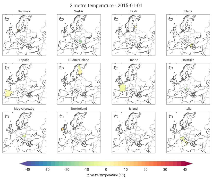
institution: ECMWFWe can now use earthkit-plots to plot the masked features, below we select the first time step and produce for the first 12 features.
[8]:
plot_data = masked_data.isel(valid_time=0)

figure = ekp.Figure(domain="Europe", size=(9, 7), rows=3, columns=4)
nmaps = figure.rows * figure.columns

for i in range(nmaps):
    subplot = figure.add_map()
    subplot.pcolormesh(plot_data.isel(NAME_LATN=i), style="2m-temperature-spectral-celsius")
    subplot.title("{NAME_LATN}")

figure.title("{variable_name} - {valid_time:%Y-%m-%d}")
figure.coastlines()
figure.borders()
figure.legend()

figure.show()
/tmp/ipykernel_1276/3206239347.py:3: DeprecationWarning: The 'size' argument is deprecated and will be removed in a future release. Use 'figsize' instead.
  figure = ekp.Figure(domain="Europe", size=(9, 7), rows=3, columns=4)
/home/docs/checkouts/readthedocs.org/user_builds/earthkit-transforms/envs/1.0.0/lib/python3.11/site-packages/cartopy/io/__init__.py:242: DownloadWarning: Downloading: https://naturalearth.s3.amazonaws.com/50m_cultural/ne_50m_admin_0_boundary_lines_land.zip
  warnings.warn(f'Downloading: {url}', DownloadWarning)
Union geometries
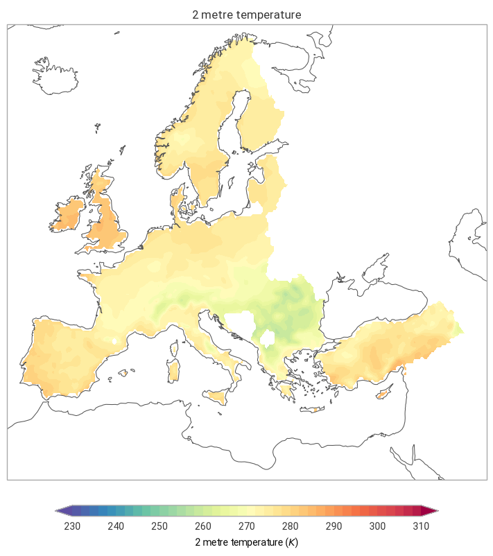
ekt.spatial.mask allows users to unify all geometries into a single feature when applying the mask via the kwarg union_geometries.
[9]:
single_masked_data = ekt.spatial.mask(era5_xr, nuts_data, union_geometries=True)
single_masked_data
[9]:
<xarray.Dataset> Size: 11MB
Dimensions:     (valid_time: 24, latitude: 201, longitude: 281)
Coordinates:
  * valid_time  (valid_time) datetime64[us] 192B 2015-01-01 ... 2015-01-01T23...
  * latitude    (latitude) float64 2kB 80.0 79.75 79.5 79.25 ... 30.5 30.25 30.0
  * longitude   (longitude) float64 2kB -10.0 -9.75 -9.5 ... 59.5 59.75 60.0
Data variables:
    t2m         (valid_time, latitude, longitude) float64 11MB dask.array<chunksize=(24, 201, 281), meta=np.ndarray>
Attributes:
    Conventions:  CF-1.8
institution: ECMWF[10]:
ekp.geo.plot(single_masked_data.mean(dim="valid_time"), domain="Europe").show()
[10]:
<earthkit.plots.components.figures.Figure at 0x76da7de85c50>