Climatology calculations¶

[1]:

from earthkit import data as ekd
from earthkit import plots as ekp
from earthkit import transforms as ekt
from earthkit.transforms._tools import earthkit_remote_test_data_file

Calculate the climatologies¶

The climatology module offers a range of methods for calculating climatological statistics. First we will use the basic methods to calculate climatological mean and standard-deviation representative of the climatology period 1991-2020.

The climatology_range must provide the start and end date for the climatology period. It can be provided as date strings which are recognised by xarray, for example "YYYY", "YYYY-MM" and "YYYY-MM-DD", or as a date objects such as datetime objects or numpy.datetime64 objects.

If the climatology range is not provided, then the whole time-period in the input data is used.

[3]:

climatology_mean = ekt.climatology.mean(era5_xr, climatology_range=("1991", "2020"))
climatology_std = ekt.climatology.std(era5_xr, climatology_range=("1991", "2020"))
print(
    f"Climatology mean = {float(climatology_mean.t2m)}\nClimatology standard deviation = {float(climatology_std.t2m)}"
)
climatology_mean

Climatology mean = 283.6854248046875
Climatology standard deviation = 5.9290385246276855

These functions are both wrappers of the base ekt.climatology.reduce function, where how is set to "mean" and "std" respectively.

Monthly quantiles¶

The API for climatology quantiles is slightly different, it requires an additional argument q which is a list of the quantiles to return. Additionally, the returned object has quantiles dimension which is for each of the quantiles returned.

[6]:

climatology_monthly_quantiles = ekt.climatology.quantiles(
    era5_xr, [0.1, 0.5, 0.9], frequency="month", climatology_range=("1991", "2020")
)
climatology_monthly_quantiles

[6]:

<xarray.Dataset> Size: 408B
Dimensions:   (quantile: 3, month: 12)
Coordinates:
  * quantile  (quantile) float64 24B 0.1 0.5 0.9
  * month     (month) int64 96B 1 2 3 4 5 6 7 8 9 10 11 12
Data variables:
    t2m       (quantile, month) float64 288B dask.array<chunksize=(1, 1), meta=np.ndarray>
Attributes:
    Conventions:             CF-1.7
    GRIB_centre:             ecmf
    GRIB_centreDescription:  European Centre for Medium-Range Weather Forecasts
    GRIB_edition:            1
    GRIB_subCentre:          0
    history:                 2024-09-02T04:48 GRIB to CDM+CF via cfgrib-0.9.1...
    institution:             European Centre for Medium-Range Weather Forecasts

Plot the output¶

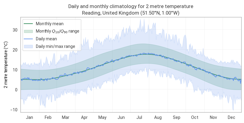
First we plot the climatology data using an earthkit-plots Climatology figure.

[7]:

chart = ekp.Climatology(wrap_time=True)

chart.fix_y_units("celsius")

# Monthly mean + q10/q90 envelope
chart.line(climatology_monthly_mean, label="Monthly mean", color="seagreen", drawstyle="spline")
chart.fill_between(
    climatology_monthly_quantiles.sel(quantile=0.1),
    climatology_monthly_quantiles.sel(quantile=0.9),
    label="Monthly $Q_{10} / Q_{90}$ range",
    color="seagreen",
    drawstyle="spline",
)

# Daily mean + min/max envelope
chart.line(
    climatology_daily_mean,
    label="Daily mean",
    color="cornflowerblue",
)
chart.fill_between(
    climatology_daily_min,
    climatology_daily_max,
    label="Daily min/max range",
    color="cornflowerblue",
)

chart.title(
    "Daily and monthly climatology for {variable_name}\n{location:%c}, {location:%C} ({latitude:%Lt}, {longitude:%Ln})"
)
chart.xticks(frequency="M", period=True)
chart.ylabel()
chart.legend()
chart.show()

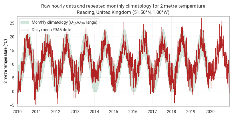
../../_images/tutorials_climatology_01-era5-climatology_20_0.png

Now we add the climatology to the background of the Timeseries plot for the daily mean on the original valid_time dimension. First we create the repeated climatology for the monthly quantiles, then we plot with earthkit-plots

[8]:

latitude = 51.5
longitude = -1.0

chart = ekp.TimeSeries()

# repeat_years tiles the month-dimensioned climatology across 2015–2017
# automatically — no dummy datetime coordinates needed.
chart.fill_between(
    climatology_monthly_quantiles.sel(quantile=0.1),
    climatology_monthly_quantiles.sel(quantile=0.9),
    units="celsius",
    label="Monthly climatology ($Q_{10} / Q_{90}$ range)",
    color="seagreen",
    drawstyle="spline",
    repeat_years=range(2010, 2020),
)

era5_daily_mean = ekt.temporal.daily_mean(era5_xr)
chart.line(
    era5_daily_mean.sel(valid_time=slice("2010", "2020")),
    units="celsius",
    label="Daily mean ERA5 data",
    color="firebrick",
    lw=1,
)

chart.title(
    "Raw hourly data and repeated monthly climatology for {variable_name}\n"
    "{location:%c}, {location:%C} ({latitude:%Lt}, {longitude:%Ln})"
)

chart.ylabel()
chart.legend()
chart.show()

../../_images/tutorials_climatology_01-era5-climatology_22_0.png

[ ]:

Climatology calculations¶

Load test data¶

Calculate the climatologies¶

Monthly climatology¶

Daily mean, min, max and standard deviation¶

Monthly quantiles¶

Plot the output¶