Anomaly calculations¶

[1]:

from earthkit import data as ekd
from earthkit import plots as ekp
from earthkit import transforms as ekt
from earthkit.transforms._tools import earthkit_remote_test_data_file

Plot the output¶

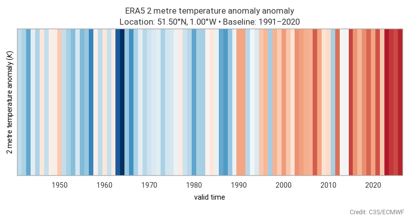
Climate stripes¶

We can use the annual anomaly to plot the climate strips for our time-series.

[8]:

chart = ekp.timeseries.stripes(anomaly_annual, cmap="RdBu_r")

chart.xticks(frequency="10Y")

chart.title("ERA5 {variable_name} anomaly\nLocation: {latitude:%Lt}, {longitude:%Ln} • Baseline: 1991–2020")
chart.attribution("Credit: C3S/ECMWF", location="lower right")

chart.show()

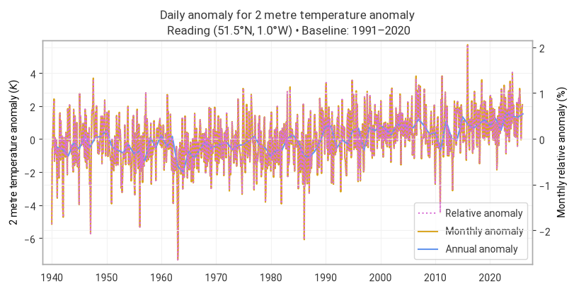
../../_images/tutorials_climatology_02-era5-anomaly_14_0.png

Traditional time-series on a single plot¶

[9]:

fig = ekp.TimeSeries()

# Add the absolute anomalies
# # Uncomment the line below to plot the anomaly calculated using the original time-dimension (e.g. daily)
# # data, but this will be very noisy and not very informative.
# fig.line(anomaly_original_time_dim, label="Original time-dimension anomaly", color="seagreen", alpha=0.5)
fig.line(anomaly_monthly, label="Monthly anomaly", color="goldenrod")
fig.line(anomaly_annual, label="Annual anomaly", color="cornflowerblue")
fig.ylabel()

ax2 = fig.ax.twinx()
ax2.plot(
    relative_anomaly_monthly["valid_time"],
    relative_anomaly_monthly["t2m"],
    label="Relative anomaly",
    color="orchid",
    linestyle=":",
)
ax2.set_ylabel("Monthly relative anomaly (%)")

handles, labels = fig.ax.get_legend_handles_labels()
handles2, labels2 = ax2.get_legend_handles_labels()
fig.ax.legend(handles2 + handles, labels2 + labels, loc="lower right")

fig.title("Daily anomaly for {variable_name}\n Reading (51.5°N, 1.0°W) • Baseline: 1991–2020")

fig.show()

../../_images/tutorials_climatology_02-era5-anomaly_16_0.png

[ ]: