Daily statistics from hourly ERA5 data

[11]:

# If first time running, uncomment the line below to install any additional dependancies
# !bash requirements-for-notebooks.sh

[12]:

from earthkit.transforms import aggregate as ek_aggregate
from earthkit import data as ek_data

from earthkit.data.testing import earthkit_remote_test_data_file
ek_data.settings.set("cache-policy", "user")

import matplotlib.pyplot as plt

Load some test data

All earthkit-climate methods can be called with earthkit-data objects (Readers and Wrappers) or with the pre-loaded xarray.

In this example we will use hourly ERA5 2m temperature data on a 0.5x0.5 spatial grid for the year 2015 as our physical data.

First we download (if not already cached) lazily load the ERA5 data (please see tutorials in earthkit-data for more details in cache management).

We inspect the data using the describe method and see we have some 2m air temperature data. For a more detailed representation of the data you can use the to_xarray method.

[13]:

# Get some demonstration ERA5 data, this could be any url or path to an ERA5 grib or netCDF file.
remote_era5_file = earthkit_remote_test_data_file("test-data", "era5_temperature_europe_2015.grib")
era5_data = ek_data.from_source("url", remote_era5_file)
# era5_data.to_xarray()
era5_data.describe()

[13]:

		level	date	time	step	paramId	class	stream	type	experimentVersionNumber
shortName	typeOfLevel
2t	surface	0	20150301,20150302,...	0,1800,...	0	167	ea	oper	an	0001

Calculate a rolling mean with a 50 timestep window

To calculate a rolling mean along the time dimension you can use the rolling_reduce function.

NOTE: An improved API to the rolling_reduce method is an ongoing task

[16]:

era5_rolling = ek_aggregate.temporal.rolling_reduce(
    era5_data, 50, how_reduce="mean", center=True,
)
era5_rolling

[16]:

<xarray.Dataset> Size: 330MB
Dimensions:     (number: 1, time: 1460, step: 1, surface: 1, latitude: 201,
                 longitude: 281)
Coordinates:
  * number      (number) int64 8B 0
  * time        (time) datetime64[ns] 12kB 2015-01-01 ... 2015-12-31T18:00:00
  * step        (step) timedelta64[ns] 8B 00:00:00
  * surface     (surface) float64 8B 0.0
  * latitude    (latitude) float64 2kB 80.0 79.75 79.5 79.25 ... 30.5 30.25 30.0
  * longitude   (longitude) float64 2kB -10.0 -9.75 -9.5 ... 59.5 59.75 60.0
    valid_time  (time, step) datetime64[ns] 12kB dask.array<chunksize=(1460, 1), meta=np.ndarray>
Data variables:
    t2m         (number, time, step, surface, latitude, longitude) float32 330MB dask.array<chunksize=(1, 1459, 1, 1, 201, 281), meta=np.ndarray>
Attributes:
    GRIB_edition:            1
    GRIB_centre:             ecmf
    GRIB_centreDescription:  European Centre for Medium-Range Weather Forecasts
    GRIB_subCentre:          0
    Conventions:             CF-1.7
    institution:             European Centre for Medium-Range Weather Forecasts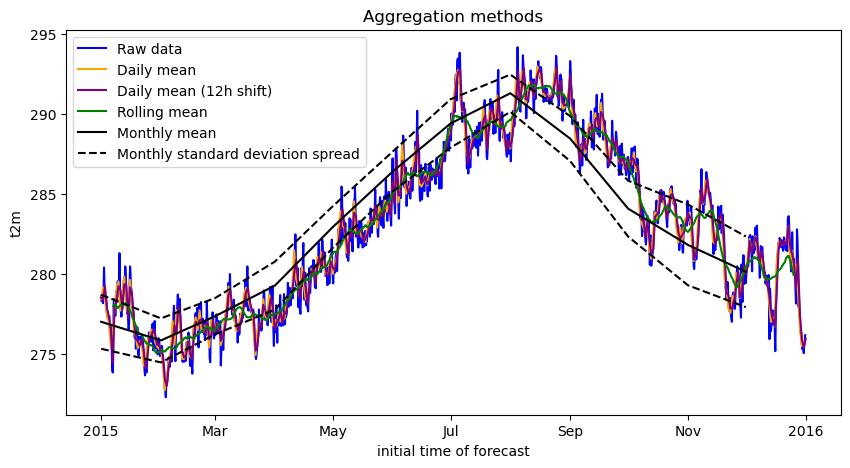
    history:                 2024-07-12T08:59 GRIB to CDM+CF via cfgrib-0.9.1...

Plot a random point location to see the different aggregation methods

[18]:

isel_kwargs = {"latitude":100, "longitude":100}

fig, ax = plt.subplots(ncols=1, nrows=1, figsize=(10,5))

era5_data.to_xarray().t2m.isel(**isel_kwargs).plot(label='Raw data', ax=ax, color='blue')
era5_daily_mean.t2m.isel(**isel_kwargs).plot(
    label='Daily mean', ax=ax, color='orange'
)

era5_daily_mean_p12.t2m.isel(**isel_kwargs).plot(
    label='Daily mean (12h shift)', ax=ax, color='purple'
)

# # To add the daily spread as orange dotted lines:
# upper_d = era5_daily_mean.t2m + era5_daily_std.t2m
# lower_d = era5_daily_mean.t2m - era5_daily_std.t2m
# upper_d.isel(**isel_kwargs).plot(ax=ax, label='Daily standard deviation spread', linestyle='--', color='orange')
# lower_d.isel(**isel_kwargs).plot(ax=ax, linestyle='--', color='orange')

# Add the rolling mean as green line:
era5_rolling.t2m.isel(**isel_kwargs).plot(label='Rolling mean', ax=ax, color='green')

# Add the monthly mean as a black solid line and spread as black dotted lines:
era5_monthly_mean.t2m.isel(**isel_kwargs).plot(label='Monthly mean', ax=ax, color='black')
upper_m = era5_monthly_mean.t2m + era5_monthly_std.t2m
lower_m = era5_monthly_mean.t2m - era5_monthly_std.t2m
upper_m.isel(**isel_kwargs).plot(ax=ax, label='Monthly standard deviation spread', linestyle='--', color='black')
lower_m.isel(**isel_kwargs).plot(ax=ax, linestyle='--', color='black')


# figure = fig[0].get_figure()
ax.legend(loc=2)
ax.set_title("Aggregation methods")
plt.show()

../../../_images/notebooks_aggregate_temporal_02-era5-daily-monthly-statistics_14_0.png

[ ]:

Daily statistics from hourly ERA5 data

Load some test data

Calculate the daily mean and standard deviation of the ERA5 data

Calculate the monthly mean and standard deviation

Calculate a rolling mean with a 50 timestep window

Account for non-UTC timezones

Plot a random point location to see the different aggregation methods