Daily statistics from six-hourly SEAS5 data
[1]:
import matplotlib.pyplot as plt
from earthkit.data.testing import earthkit_remote_test_data_file

from earthkit import data as ekd
from earthkit.transforms import aggregate as ekt

ekd.settings.set("cache-policy", "user")
Load some test data
All earthkit-transforms methods can be called with earthkit-data objects (Readers and Wrappers) or with the pre-loaded xarray.
In this example we will use three initialisation of the SEAS5 2m temperature data on a 1.x1. spatial grid. The temporal resolution is 6 hourly, and we have the forecasts for January, February and March 2015.
First we download (if not already cached) and lazily load the SEAS5 data (please see tutorials in earthkit-data for more details in cache management).
We convert the data to an xarray.Dataset object with some additional options better suited for the data we’re handling.
[2]:
# Get some demonstration ERA5 data, this could be any url or path to an ERA5 grib or netCDF file.
remote_seas5_file = earthkit_remote_test_data_file("seas5_2m_temperature_201501-201503_europe_1deg.grib")
seas5_data = ekd.from_source("url", remote_seas5_file)
seas5_xr = seas5_data.to_xarray(time_dim_mode="forecast", add_valid_time_coord=True).rename({"2t": "t2m"})
seas5_xr
[2]:
<xarray.Dataset> Size: 182MB
Dimensions:                  (number: 25, forecast_reference_time: 3,
                              step: 239, latitude: 31, longitude: 41)
Coordinates:
  * number                   (number) int64 200B 0 1 2 3 4 5 ... 20 21 22 23 24
  * forecast_reference_time  (forecast_reference_time) datetime64[us] 24B 201...
  * step                     (step) timedelta64[us] 2kB 0 days 06:00:00 ... 5...
    valid_time               (forecast_reference_time, step) datetime64[ns] 6kB ...
  * latitude                 (latitude) float64 248B 70.0 69.0 ... 41.0 40.0
  * longitude                (longitude) float64 328B -10.0 -9.0 ... 29.0 30.0
Data variables:
    t2m                      (number, forecast_reference_time, step, latitude, longitude) float64 182MB ...
Attributes: (12/14)
    param:        2t
    paramId:      167
    class:        c3
    stream:       mmsf
    levtype:      sfc
    type:         fc
    ...           ...
    time:         0
    origin:       ecmf
    domain:       g
    method:       1
    Conventions:  CF-1.8
institution: ECMWFCalculate the daily median of the Seasonal Forecast data
In this first example we will handle the forecast initialisations independently, i.e. return the daily median of the 3 different forecasts. To do this we must specify that the time-dimension we wish to calculate the aggregation over is the “step” dimension.
[3]:
seas_daily_median_by_step = ekt.temporal.daily_median(seas5_xr, time_dim="step")
seas_daily_median_by_step.coords["valid_time"] = (
    seas_daily_median_by_step["forecast_reference_time"] + seas_daily_median_by_step["step"]
)
seas_daily_median_by_step
/tmp/ipykernel_1202/1229309637.py:1: DeprecationWarning: The function 'daily_median' from the legacy aggregate module is deprecated and will be removed in version 2.X of earthkit.transforms. Use 'earthkit.transforms.temporal.daily_median' instead.
  seas_daily_median_by_step = ekt.temporal.daily_median(seas5_xr, time_dim="step")
[3]:
<xarray.Dataset> Size: 46MB
Dimensions:                  (step: 60, number: 25, forecast_reference_time: 3,
                              latitude: 31, longitude: 41)
Coordinates:
  * step                     (step) timedelta64[us] 480B 0 days 06:00:00 ... ...
    valid_time               (forecast_reference_time, step) datetime64[us] 1kB ...
  * number                   (number) int64 200B 0 1 2 3 4 5 ... 20 21 22 23 24
  * forecast_reference_time  (forecast_reference_time) datetime64[us] 24B 201...
  * latitude                 (latitude) float64 248B 70.0 69.0 ... 41.0 40.0
  * longitude                (longitude) float64 328B -10.0 -9.0 ... 29.0 30.0
Data variables:
    t2m                      (step, number, forecast_reference_time, latitude, longitude) float64 46MB ...
Attributes: (12/14)
    param:        2t
    paramId:      167
    class:        c3
    stream:       mmsf
    levtype:      sfc
    type:         fc
    ...           ...
    time:         0
    origin:       ecmf
    domain:       g
    method:       1
    Conventions:  CF-1.8
institution: ECMWF[4]:
seas5_daily_median_by_vt = ekt.temporal.daily_median(seas5_xr, time_dim="valid_time")
seas5_daily_median_by_vt
/tmp/ipykernel_1202/3673849465.py:1: DeprecationWarning: The function 'daily_median' from the legacy aggregate module is deprecated and will be removed in version 2.X of earthkit.transforms. Use 'earthkit.transforms.temporal.daily_median' instead.
  seas5_daily_median_by_vt = ekt.temporal.daily_median(seas5_xr, time_dim="valid_time")
[4]:
<xarray.Dataset> Size: 30MB
Dimensions:    (date: 119, number: 25, latitude: 31, longitude: 41)
Coordinates:
  * date       (date) datetime64[s] 952B 2015-01-01 2015-01-02 ... 2015-04-29
  * number     (number) int64 200B 0 1 2 3 4 5 6 7 8 ... 17 18 19 20 21 22 23 24
  * latitude   (latitude) float64 248B 70.0 69.0 68.0 67.0 ... 42.0 41.0 40.0
  * longitude  (longitude) float64 328B -10.0 -9.0 -8.0 -7.0 ... 28.0 29.0 30.0
Data variables:
    t2m        (date, number, latitude, longitude) float64 30MB 269.2 ... 282.2
Attributes: (12/14)
    param:        2t
    paramId:      167
    class:        c3
    stream:       mmsf
    levtype:      sfc
    type:         fc
    ...           ...
    time:         0
    origin:       ecmf
    domain:       g
    method:       1
    Conventions:  CF-1.8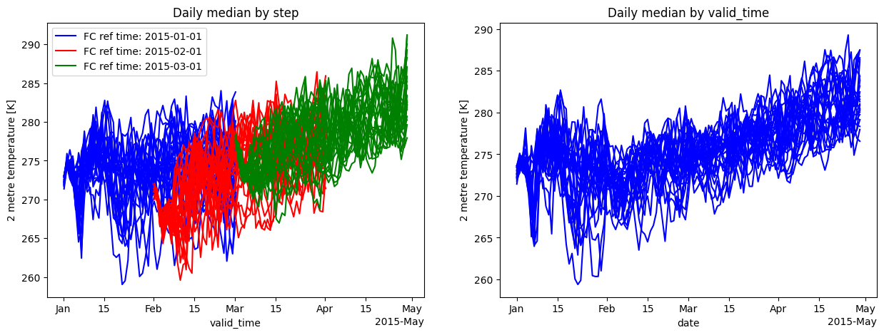
institution: ECMWFPlot a random point location to see the different aggregation methods
[5]:
isel_kwargs = {"latitude": 20, "longitude": 20}

fig, axes = plt.subplots(ncols=2, nrows=1, figsize=(15, 5))

forecast_colours = ["blue", "red", "green"]

# era5_data.to_xarray().t2m.isel(**isel_kwargs).plot(label='Raw data', ax=ax)
f_kwargs = {"label": "Daily median over step"}

for itime in range(3):
    for number in range(25):
        t_data = seas_daily_median_by_step.t2m.isel(**isel_kwargs, number=number, forecast_reference_time=itime)
        if number == 0:
            extra_kwargs = {"label": f"FC ref time: {str(t_data.forecast_reference_time.values)[:10]}"}
        else:
            extra_kwargs = {}
        t_data.plot(x="valid_time", ax=axes[0], color=forecast_colours[itime], **extra_kwargs)
axes[0].legend(loc=2)
axes[0].set_title("Daily median by step")

for number in range(25):
    t_data = seas5_daily_median_by_vt.t2m.isel(**isel_kwargs, number=number)
    extra_kwargs = {}
    t_data.plot(x="date", ax=axes[1], color=forecast_colours[0], **extra_kwargs)

axes[1].set_title("Daily median by valid_time")

plt.show()
[ ]: